dammix
Manual
Introduction
DAMMIX reconstructs the shape of an unknown component in an evolving system and estimates the volume fractions of all components at each measured condition. The initial and final states of the system are assumed to be known or approximated from theoretical or experimental scattering data.
The program uses an ab initio bead modeling approach similar to DAMMIF and searches for the most compact bead model whose linear combinations with the known initial and final states best fit the SAXS data. Volume fractions are determined using the same algorithm as in OLIGOMER.
Running DAMMIX
Command-Line
Usage:
$ dammix [OPTIONS] [SASDATA(S)]
OPTIONS known by DAMMIX are described in next section, the optional argument ‘ DATAFILE(S) ‘ in the section on input files. In general, command-line options can be used to make choices about the properties of the particle to reconstruct, while the interactive configuration is used to govern the annealing process. If neither OPTIONS nor DATAFILE(S) is given, the configuration is done in full interactive mode.
Arguments and Options
DAMMIX accepts the following command line arguments:
| Argument | Description |
|---|---|
| SASDATA(S) | Relative or absolute paths to experimental SAS data (.dat) |
The first and second positional arguments define the initial and final system states. Both these states can be provided either as experimental SAS data (.dat) or as atomic model in .pdb or .cif format. If an atomic model is provided, the corresponding theoretical scattering curve is calculated and used as the known component of the system.
All remaining positional arguments (3rd, 4th, …) are considered experimental
curves for intermediate conditions; DAMMIX reconstructs the unknown component
and estimates volume fractions for each curve. For two-component mixtures,
set the second argument to none (this exact string).
DAMMIX recognizes the following command-line options. Mandatory arguments to long options are mandatory for short options too.
| Short Option | Long Option | Description |
|---|---|---|
| -q | --quiet | Suppress screen output, write a .log-file only. By default, all runtime information is printed to screen and the .log-file. |
| --seed=<INT> | Set the seed for the random number generator | |
| -u | --unit=<u|1|2|3|4> | Define angular units of the experimental SAS data (.dat) files. |
| -p | --prefix=<PREFIX> | Prefix to prepend to output filenames. May include absolute or relative paths, all directory components must exist. Default is ‘dammif’. |
| --model-format=<FMT> | Format of 3D models, one of: cif, pdb (default: cif) | |
| -a | --anisometry=<NAME> | If, due to prior studies, it is known that the particle’s shape shall be eitherPROLATEorOBLATE, one may use the anisometry option to enforce a penalty on particles that do not correspond with the expected anisometry. By default, anisometry is ‘UNKNOWN’. |
| -s | --symmetry=<NAME> | Specify the symmetry to enforce on the particle (P_n_,n=1, …, 19 and P_n_2,n=2, …, 12). Cubic and icosahedral symmetries are not available. By default, no symmetry is enforced (P1). |
| -m | --mode=<MODE> | Configuration of the annealing procedure, one of FAST (bigger beads, cooling down quickly), SLOW (smaller beads, cooling down slowly), or INTERACTIVE. Default is ‘INTERACTIVE’. See example. |
| --constant=<VALUE> | Specify a user defined constant to subtract; 0 to disable constant subtraction. If unspecified, a constant to subtract is automatically determined. | |
| --volume | Activation of the manual input for excluded Porod volumes for each individual input curve. | |
| --max-bead-count=<NUMBER> | Maximum number of beads in search volume (unlimited if undefined). | |
| -h | --help | Print a summary of arguments, options, and exit. |
| -v | --version | Print version information and exit. |
Interactive Configuration
If the optional arguments ' DATAFILE(S)` are omitted, settings available
through command-line arguments and options may also be configured
interactively as shown in the table below. Otherwise these questions are
skipped.
An interactive answers file (.ans) may be used to record and replay configurations, enabling repeatable runs without re-entering parameters.
| Screen Text | Default | Description |
|---|---|---|
| Number of experimental curves? | 5 | Total number of experimental curves including the initial and final states of the system. Defualt value is set to 5. |
| DATA input files? | N/A | Same as DATAFILE argument. The first argument corresponds to the initial state of the system (e.g. monomer), the second argument to the final state (e.g. aggregate), one can use for them both experimental data files (DAT) or PDB models (PDB) formats. The rest of the agruments should represent experimental scattering curves. |
| Angular unit? | UNKNOWN | Same as the unit option. |
| Output file prefix? | dammix | Same as the prefix option. |
| Create pseudo chains in PDB output? | NO | Same as the chained option. |
| Expected particle symmetry? | P1 | Same as the symmetry option. |
| Expected particle anisometry? | UNKNOWN | Same as the anisometry option. |
| Simulated annealing setup? | SLOW | Same as the mode option. |
In INTERACTIVE mode a list of parameters governing the annealing process may be fine-tuned:
| Screen Text | Default | FAST-mode Setting | SLOW-mode Setting | Description |
|---|---|---|---|---|
| Dummy atom radius? [1.0-?] [Angstrom] | var | var | var | The estimate for the dummy atom radius is based on_D~max~_to result in a search volume of about 2.000 (FAST-mode) to about 10.000 (SLOW-mode) beads. The smaller this radius is set, the more beads are generated, the slower the process. |
| Maximum number of spherical harmonics? [1-50] | 20 | 15 | 20 | The more harmonics, the more accurate the reconstruction becomes, but the slower the process. Very elongated particles may require up to 50 harmonics, quick screening can be done as low as 10-15. The default values may be adjusted by shape classification. |
| Number of knots in the curve to fit? [1-?] | var | var | var | Experimental data is smoothed by spline interpolation before fitting. This defines the number of supporting points of the spline. By default, twice the number of Shannon Channels is used, but a minimum of 20. |
| Curve weighting function? Select one of: [l]og, [p]orod, [e]mphasised porod, [n]one | emph. porod | emph. porod | emph. porod | Weighting function to ensure a better fit at lower angles. If unsure, use the default. |
| Initial random seed? | var | var | var | To reproduce results, re-use the random seed. Default value is time-based. If multiple runs of DAMMIX shall be started at the same time, use an input file with different random seeds. |
| Maximum number of temperature steps in annealing procedure? [1-?] | 200 | 200 | 400 | Stop if simulated annealing is not finished after this many steps. The more iterations per step and the slower the system is cooled, the more temperature steps are required. |
| Maximum number of iterations within a single temperature step? [1-?] | 200.000 | 20.000 | 100.000 | Finalize temperature step and cool after this many iterations at the latest. |
| Maximum number of successes per temperature step before temperature is decreased? [1-?] | 20.000 | 2.000 | 10.000 | Finalize temperature step and cool after at most this many successful phase changes. |
| Minimum number of successes per temperature step before temperature is decreased? [1-?] | 200 | 20 | 50 | Stop if not at least this many successful state changes within a single temperature step can be done. |
| Temperature schedule factor? [0.0-1.0) | 0.95 | 0.9 | 0.95 | Factor by which the temperature is decreased; 0.95 is a good average value. Faster cooling for smaller systems is possible (0.9), but slower cooling (0.99) needs to be applied more often. The default factor is increased for extended particles. |
| Rg penalty weight? [0.0-…) | 0.001 | 0.001 | 0.001 | How much the R~g~Penalty shall influence the acceptance or rejection of phase changes. A value of 0.0 disables the penalty. If unsure, use the default value. |
| Center penalty weight? [0.0-…) | 0.00001 | 0.00001 | 0.00001 | How much the Center Penalty shall influence the acceptance or rejection of phase changes. A value of 0.0 disables the penalty. If unsure, use the default value. |
| Looseness penalty weight? [0.0-…) | 0.01 | 0.01 | 0.01 | How much the Looseness Penalty shall influence the acceptance or rejection of phase changes. A value of 0.0 disables the penalty. If unsure, use the default value. If unlike smooth surfaces and sharp edges are observed, try decreasing this penalty weight. |
| Anisometry penalty weight? [0.0-…) | 0.0/0.5 | 0.0/0.5 | 0.0/0.5 | How much the Anisometry Penalty shall influence the acceptance or rejection of phase changes. A value of 0.0 disables the penalty. If unsure, use the default value, 0.0 if no anisometry was specified, 0.5 otherwise. |
| Minimum volume fraction penalty weight? [0.0-…) | 0.0/0.5 | 0.0/0.5 | 0.0/0.5 | To keep the minimum volume fraction of unknown component not below 3% (over all curves). A value of 0.0 disables the penalty. If unsure, use the default value. If the volume fractions of uknown component are too high, try decreasing this penalty weight. |
| Oligomer volume penalty weight? [0.0-…) | 0.0/0.5 | 0.0/0.5 | 0.0/0.5 | Applied for two-components systems when the oligomeric state of the restoring component is known. A value of 0.0 disables the penalty. If unsure, use the default value. |
Runtime Output
On runtime, two lines of output will be generated for each temperature step:
Step:    4, T: 0.238E-04, 723/2500, Succ: 2000, Eval: 13840, CPU: 00:00:15
 Rf: 0.1954, Los: 0.10, Rg: 0.27730E+01, Cen: 3.04, Ani: 0.00, Mfr: 0.00,
 Vol: 0.45011E+01 Fit: 0.2048
The fields can be interpreted as follows, top-left to bottom-right:
| Field | Description |
|---|---|
| Step | Step number. Starts at 1, increases monotonically. |
| T | Temperature measure, starts at an arbitrary high value, decreases each step by the temperature schedule factor. |
| N/M | N beads in phase particle in M beads overall. |
| Succ | Number of successful phase changes in this temperature step. Limited by the minimum and maximum number of successes. The number of successes should slowly decrease, the first couple of steps should be terminated by the maximum number of successes criterion. If instead the maximum number of iterations per step are done, or the number of successes drops suddenly by a large amount, the system should probably be cooled more slowly. |
| Eval | Accumulated number of function evaluations. |
| CPU | Elapsed wall-clock time since the annealing procedure was started. |
| Rf | Goodness of overall fit of simulated data versus experimental data (to all experimental data curves), does not take penalties into account. |
| Los | Contribution of Looseness Penalty, not taking the Looseness Penalty Weight into account. |
| Rg | Contribution of \(R_g\) Penalty, not taking the \(R_g\) Penalty Weight into account. |
| Cen | Contribution of Center Penalty, not taking the Center Penalty Weight into account. |
| Ani | Contribution of Anisometry Penalty, not taking the Anisometry Penalty Weight into account. |
| Mfr | Contribution of Minimum Fraction Penalty for the uknown component, not taking the Minimum Fraction Penalty Weight into account. |
| Vol | Contribution of Volume Penalty for the uknown component (to be used for two-component mixtures when the oligomeric state of the restoring component is known), not taking the Volume Penalty Weight into account. |
| Fit | A function ofRfincluding all penalties and their respective weights. Decreases towards zero, the smaller the value, the better the fit. |
Graphical Interface
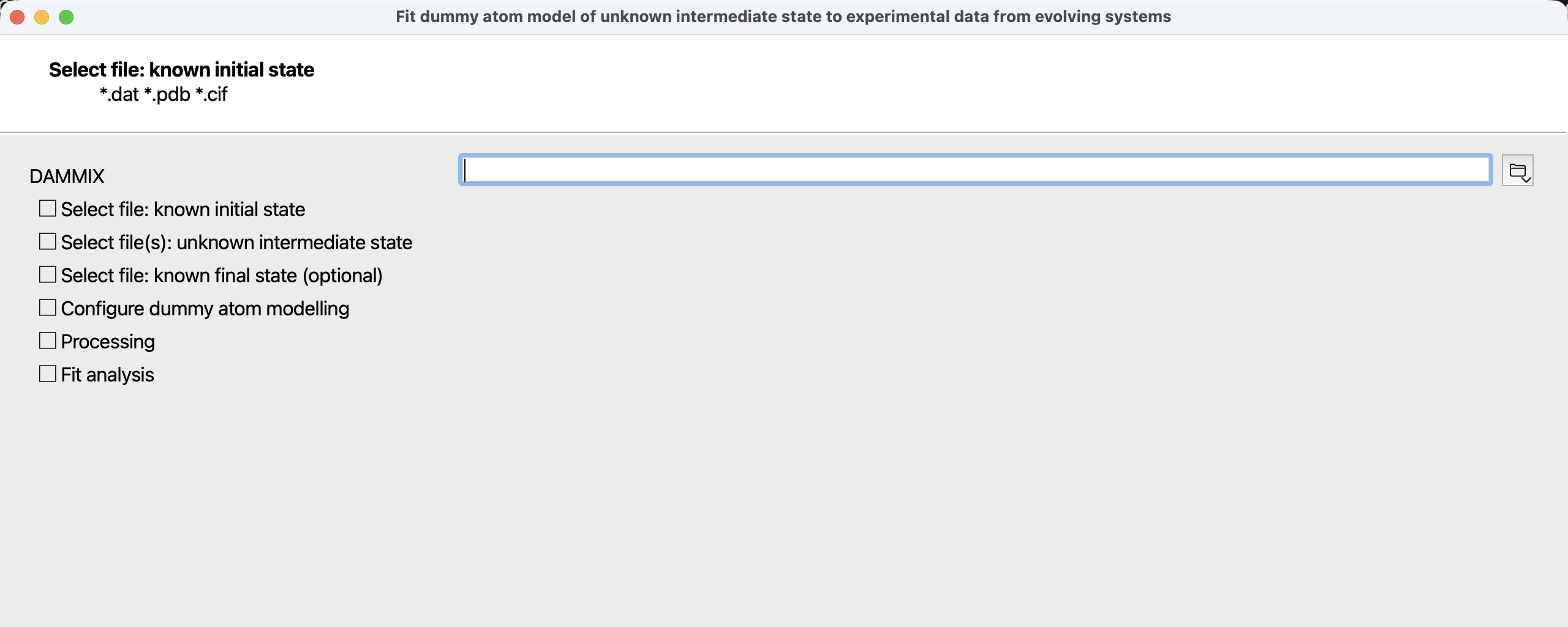 Figure 1: first page of the DAMMIX wizard when started from the ATSAS Application Launcher.
As an alternative to usage from the command-line, DAMMIX may also be run as a wizard from the ATSAS Application Launcher.
This wizard allows convenient configuration of the arguments and options and interactive configuration as outlined in the command-line section. After completion of all calculations, the fits can be inspected and the output files saved.
DAMMIX Input Files
CRYSOL reads one or more experimental SAS data (.dat) files.
The first two arguments may alternatively also be atomic models in either .pdb .cif or .ent format.
See Arguments and Options for a note on the implied meaning of positional arguments.
DAMMIX Output Files
With each succesful run, DAMMIX creates a set of output files, each filename starts with a customizable prefix that gets an extension appended. If a prefix has been used before, existing files will be overwritten without further note.
| Extension | Description |
|---|---|
| .log | A copy of the screen output |
| -1.pdb or -1.cif | The model is proveded in either PDB or mmCIF format, depending on the model-format option. |
| .fit | Fits from the three (or two)-component mixtures (using the restored shape of the unknown component and restored volume fractions of all components) versus each individual experimental data curve (except the first two curves in the command line argument list that correspond to the known system states). |
| .dat | Two files: components_best.dat and fractions_best.dat that contain the restored scattering patterns from the components of the mixture and the restored volume fractions of the components for each experimental curve. |
Examples
Please note that the prefixes in the examples may be chosen arbitrarily. The values below are chosen for maximum clarity only.
Intermediate states for time-resolved data series
Use DAMMIX in FAST mode to obtain a first model quickly for 14 hours insulin fibrillation time seria (the initial and final states of the system corresponds to r1.dat and r14.dat):
$ dammix r1.dat r14.dat r2.dat r3.dat r4.dat r5.dat r6.dat r7.dat r8.dat r9.dat r10.dat r11.dat r12.dat r13.dat --prefix=insulin --mode=fast --unit=2
Monomer-multimer equilibrium
Use DAMMIX in SLOW mode to get an improved reconstruction for two-component concentration dependent NGF seria (mixture of dimers and dimers of dimers), the initial state is calculated from ngf.pdb (dimer model), the final state is described by ‘none’ in order to account for two-component mixture:
$ dammix ngf.pdb none ngf1.dat ngf2.dat ngf3.dat ngf4.dat ngf5.dat --prefix=ngf --mode=slow --unit=1
Multiple assembly states
For best results, run DAMMIX in INTERACTIVE mode, customizing annealing parameters as required. This is an example of multiple assembly states of lumazine synthase that forms icosahedral capsids of T1 (Dmax=18 nm) and T3 types (Dmax=30 nm), the restored shape corresponds to the dissociated free facets of the capsids:
$ dammix t1.pdb t3.pdb lym1.dat lym2.dat lym3.dat lym4.dat lym5.dat lym6.dat lym7.dat lym8.dat lym9.dat lym10.dat --prefix=lym --mode=interactive