sasrefcv
Manual
The following describes SASREFCV, the contrast-variation extension of the rigid body modelling program SASREF. This manual provides details of the interactive dialog, required input files, and produced output files.
Introduction
SASREFCV performs quaternary structure modelling of a complex particle formed by subunits with known atomic structures against contrast-variation SAS data. Multiple data sets can be fitted simultaneously, e.g. different D2O solvent content and/or perdeuteration, optionally together with X-ray curves. Symmetry can be applied globally and also specified for individual subunits and curves.
A simulated annealing protocol is employed to construct an interconnected ensemble of subunits without steric clashes, while minimizing the discrepancy between experimental scattering data and the predicted curves from the appropriate subunit assemblies.
For further details of the rigid body modelling approach, please refer to the SASREF manual.
Running sasrefcv
Command-Line
Usage:
$ sasrefcv [OPTIONS]
SASREFCV is configured in interactive mode; command-line options are used to supplement the run.
Arguments and Options
SASREFCV recognizes the following command-line options. Mandatory arguments to long options are mandatory for short options too.
| Short Option | Long Option | Description |
|---|---|---|
| --seed=<INT> | Set the seed for the random number generator | |
| --model-format=<FMT> | Format of 3D models, one of: cif, pdb (default: cif) | |
| --alternative-names | Enable alternative atom naming for all atomic structure files; default: disabled. | |
| --implicit-hydrogen=<N> | Set this to a value N>=0 to override ‘unable to determine number of hydrogens’ errors. | |
| --sub-element=<NAME> | Set this to a valid element to override ‘unable to determine element’ errors. | |
| -h | --help | Print a summary of arguments, options, and exit. |
| -v | --version | Print version information and exit. |
Interactive Configuration
SASREFCV runs in dialog mode. A substantial part of the setup is provided through configuration files.
There are two modes, EXPERT and USER. In EXPERT mode, more parameters can be changed. In USER mode, fewer questions are asked and defaults are used for most parameters. The default values are identical in both modes.
An interactive answers file (.ans) may be used to record and replay configurations, enabling repeatable runs without re-entering parameters.
| Screen text | Mode | Default value | Description |
|---|---|---|---|
| Computation mode (User or Expert) | U|E | USER | Mode selection. |
| Log file name | U|E | N/A | Project identifier, used as prefix for output files. |
| Enter project description | U|E | N/A | Free text stored in the log file. |
| Symmetry: Pn(2) (n=2-9) | U|E | P1 | Master symmetry. Subunits and curves may use lower symmetry. Supported symmetries are P1, P2-P9, P222, and P32-P92. |
| File name with curves info | U|E | N/A | Configuration file for scattering profiles to fit. |
| File name with smearing parameters | U|E | empty | Optional resolution-smearing settings (Resolution function (.res)). If no file is given, smearing is disabled. |
| File name with subunits info | U|E | N/A | Configuration file for atomic models. |
| File name with cross-dependencies | U|E | N/A | Configuration file defining which subunits contribute to each curve. |
| Cross penalty weight | E | 10.0 | Weight of steric-overlap penalty in mutation acceptance. |
| Disconnectivity penalty weight | E | 10.0 | Weight of connectivity penalty in mutation acceptance. |
| File name, contacts conditions, CR for none <.cnd> | U|E | empty | Optional distance restraints file. |
| Contacts penalty weight | E | 10.0 | Weight for contact-restraint violations. Asked only if a contacts file is provided. |
| Expected particle shape: Prolate, Oblate, or Unknown | U|E | UNKNOWN | Optional anisometry restraint type. |
| Anisometry penalty weight | E | 1.0 | Weight of anisometry penalty. Skipped if shape is UNKNOWN. |
| Expected direction of anisometry: aLong Z, aCross Z, or Unknown | U|E | UNKNOWN | Asked only if shape is known and symmetry is P2. |
| Shift penalty weight | E | 1.0 | Weight for displacement of the full model from origin. |
| Spatial step in angstroems | E | 5.0 | Max random translation per mutation; asked per subunit. |
| Angular step in degrees | E | 20.0 | Max random rotation per mutation; asked per subunit. |
| Initial annealing temperature | E | 10.0 | Starting temperature of simulated annealing. |
| Annealing schedule factor | E | 0.9 | Cooling factor per temperature step. |
| Max # of iterations at each T | E | var | Default is 5000 * total number of subunits. |
| Max # of successes at each T | E | var | Default is 500 * total number of subunits. |
| Min # of successes to continue | E | var | Default is 50 * total number of subunits. |
| Max # of annealing steps | E | 100 | Hard stop for annealing steps. |
Runtime Output
On runtime, two lines of output are generated for each temperature step:
j:   4 T: 0.729E+01 Suc:  1000 Eva:    12497 CPU:  0.208E+03 F:99.4301 Pen: 13.803
The best chi^2 values:11.64871 5.96331
The fields can be interpreted as follows:
| Field | Description |
|---|---|
| j | Step number. Starts at 1 and increases monotonically. |
| T | Temperature value, reduced each step by the annealing schedule factor. |
| Suc | Number of successful mutations in the current temperature step. |
| Eva | Accumulated number of function evaluations. |
| CPU | Elapsed wall-clock time since start of annealing. |
| F | Best target function value obtained so far. |
| Pen | Total penalty value of the best target function. |
| The best chi^2 values | \(\chi^2\) values for each input curve in the best current model. |
Graphical Interface
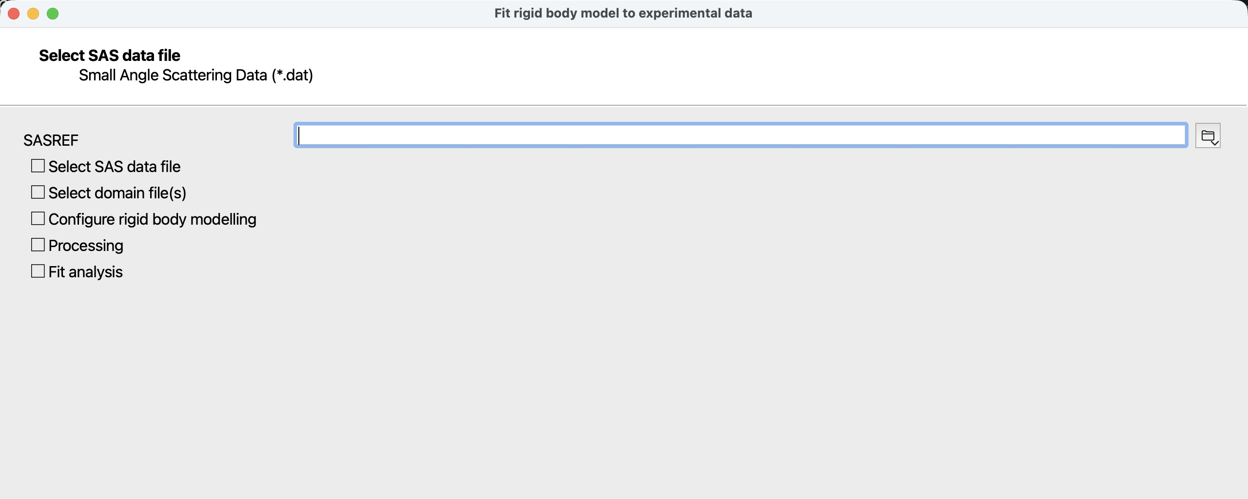 Figure 1: first page of the SASREFCV wizard when started from the ATSAS Application Launcher.
As an alternative to command-line usage, SASREFCV may also be run from the ATSAS Application Launcher.
The wizard guides the same interactive configuration and can simplify preparation of selected input files. After calculations complete, fits can be inspected in DATCMP and output files can be saved.
sasrefcv Input Files
Three compulsory configuration files are required:
Data control file
- The first row shall indicate the total number \(K\) of rows following
- \(K\) rows follow; each row has 8 whitespace-separated values/columns
Values/columns for each data row, in order:
| Column | Description | Valid values |
|---|---|---|
| 1 | File name with experimental SAS data (.dat). | An existing file name without whitespace. |
| 2 | D2O fraction in solvent, or -1.0 for X-ray data | -1.0, [0.0-1.0] |
| 3 | Symmetry for this construct under this condition | Pn, Pn2, with n=1,…,9 |
| 4 | Define angular units of the experimental SAS data (.dat). | 1, 2, 3, 4 |
| 5 | Fraction of the curve to be fitted | [0.1-1.0] |
| 6 | Setting number of an optional Resolution function (.res) | 0-15 |
| 7 | Weight of this curve in the target function | [0.0-1.0] |
| 8 | If Y, a constant background is adjusted automatically | Y|N |
See below for an example.
Subunits control file
The subunits control file describes the rigid bodies:
- The first row shall indicate the total number \(M\) of rows following
- \(M\) rows follow; each row has 4 whitespace-separated values/columns
Values/columns for each data row, in order:
| Column | Description | Valid values |
|---|---|---|
| 1 | Model file name (PDB or mmCIF) | An existing file name without whitespace. |
| 2 | Whether to shift the subunit to origin at initialization | Y|N |
| 3 | Movement limitations: - N = none - F = fixed - X = along X only - Y = along Y only - Z = along Z only - D = along (1,1,1) only |
[N/F/X/Y/Z/D] |
| 4 | Symmetry applied to this subunit | Pn, Pn2, with n=1,…,9 |
See below for an example.
Cross-correlation file
The cross-correlation file ties the experimental data and subunits together. It contains a matrix with \(M\) columns and \(K\) rows, where \(M\) is the number of subunits and \(K\) is the number of curves.
Entry (i,j) of this matrix specifies the contribution of the i-th subunit to the j-th data set.
For SANS curves the matrix value ([0.0-1.0 or -1.0]) is the subunit perdeuteration (level of D2O in expression medium); -1.0 means the subunit is not present in that construct. For X-ray curves, use 0.0 if the subunit is present, -1.0 otherwise.
See below for an example.
Distance restraints
Distance restraints may be imposed via an optional contacts conditions file:
dist 7.0
1 0 0 2 1 1
dist 5.0
2 0 0 3 1 1
dist 7.0
1 342 342 2 25 25
1 350 350 2 17 17
dist 6.0
1 290 297 2  64 79
dist 7.0
1 1 0 3 1 0
dist 7.0 means that the minimum distance between CA atoms of selected residue
ranges (or P atoms in nucleotides) should not exceed 7 \(\text{\AA}\).
In a line without dist, the 1st and 4th values are ordinal subunit numbers.
The 2nd-3rd and 5th-6th values specify residue ranges in first and second
subunits, respectively; 0 means the last residue/nucleotide.
If multiple alternatives are listed after one dist line, the smallest
alternative distance is compared to the threshold.
Please refer to the SASREF manual for details.
Important (new as of ATSAS-4.0): in the presence of symmetry, subunit numbering differs from older versions. First all symmetry mates of subunit 1 are listed, then of subunit 2, and so on.
sasrefcv Output Files
After each simulated annealing step, SASREFCV writes output files using the log-file prefix. Existing files with the same prefix are overwritten.
| Extension | Description |
|---|---|
| .log | Copy of screen output |
| .pdb or .cif | Current complex model in PDB or mmCIF format (depends on model-format). |
| -i.fit | Fit for the i-th input curve. |
Examples
Building a Complex against X-ray and Contrast Variation
SANS Data Sets A simulated example of a T7 DNA Polymerase ternary complex with DCTP (PDB entry 1t8e). Atomic coordinates of the three subunits are in:
phsave1.pdb   -   Polymerase
phsave2.pdb   -   DCTP
phsave3.pdb   -   DNA
Simulated SAS data contain 17 curves: 2 X-ray profiles (entire complex and binary construct without DNA) plus 15 neutron curves from the complex (series of D2O content 0, 40, 55, 70, 100% for each of three DCTP perdeuteration levels: 0, 50, 100%).
| File name | Description | D2O content |
|---|---|---|
| x-prot.dat | X-ray protein complex | – |
| x-compl.dat | X-ray, ternary complex | – |
| complh_0.dat | ternary complex with protonated DCTP | 0% |
| complh_40.dat | 40% | |
| complh_55.dat | 55% | |
| complh_70.dat | 70% | |
| complh_100.dat | 100% | |
| compl50d_0.dat | 50% deuterated DCTP | 0% |
| compl50d_40.dat | 40% | |
| compl50d_55.dat | 55% | |
| compl50d_70.dat | 70% | |
| compl50d_100.dat | 100% | |
| compl100d_0.dat | fully deuterated DCTP | 0% |
| compl100d_40.dat | 40% | |
| compl100d_55.dat | 55% | |
| compl100d_70.dat | 70% | |
| compl100d_100.dat | 100% |
Content of the data control file, curves.con:
17
x-prot.dat       -1.00 P1 1 1.0 0 1.0 y
x-compl.dat      -1.00 P1 1 1.0 0 1.0 y
complh_0.dat      0.00 P1 1 1.0 0 1.0 y
complh_40.dat     0.40 P1 1 1.0 0 1.0 y
complh_55.dat     0.55 P1 1 1.0 0 1.0 y
complh_70.dat     0.70 P1 1 1.0 0 1.0 y
complh_100.dat    1.00 P1 1 1.0 0 1.0 y
compl50d_0.dat    0.00 P1 1 1.0 0 1.0 y
compl50d_40.dat   0.40 P1 1 1.0 0 1.0 y
compl50d_55.dat   0.55 P1 1 1.0 0 1.0 y
compl50d_70.dat   0.70 P1 1 1.0 0 1.0 y
compl50d_100.dat  1.00 P1 1 1.0 0 1.0 y
compl100d_0.dat   0.00 P1 1 1.0 0 1.0 y
compl100d_40.dat  0.40 P1 1 1.0 0 1.0 y
compl100d_55.dat  0.55 P1 1 1.0 0 1.0 y
compl100d_70.dat  0.70 P1 1 1.0 0 1.0 y
compl100d_100.dat 1.00 P1 1 1.0 0 1.0 y
Content of the subunits control file, subunits.con:
3
phsave1.pdb Y F P1
phsave2.pdb Y N P1
phsave3.pdb Y N P1
Content of the cross-correlation file, table.con:
0.0  0.0 -1.0
0.0  0.0  0.0
0.0  0.0  0.0
0.0  0.0  0.0
0.0  0.0  0.0
0.0  0.0  0.0
0.0  0.0  0.0
0.0  0.5  0.0
0.0  0.5  0.0
0.0  0.5  0.0
0.0  0.5  0.0
0.0  0.5  0.0
0.0  1.0  0.0
0.0  1.0  0.0
0.0  1.0  0.0
0.0  1.0  0.0
0.0  1.0  0.0
A listing of questions/answers for a sample USER-mode run:
 Computation mode (User or Expert) ...... <         User >:
 Log file name .......................... <         .log >: test1
 Enter project description .............. : T7 DNA POLYMERASE WITH DCTP, 17 curves
 Symmetry: Pn(2) (n=2-9) ................ <           P1 >:
 File name with curves info ............. <         .con >: curves
 File name with smearing parameters ..... <         .res >:
 File name with subunits info ........... <         .con >: subunits
 File name with cross-dependencies ...... <         .con >: table
 File name, contacts conditions, CR for none <         .cnd >:
 Expected particle shape: <P>rolate, <O>blate,
  or <U>nknown .......................... <      Unknown >:
 ...