peak
Manual
The following sections describe the purpose of PEAK and the file formats it can work with.
Introduction
PEAK is a lightweight data analysis tool to identify partial ordering of samples from experimental SAS data (.dat) files.
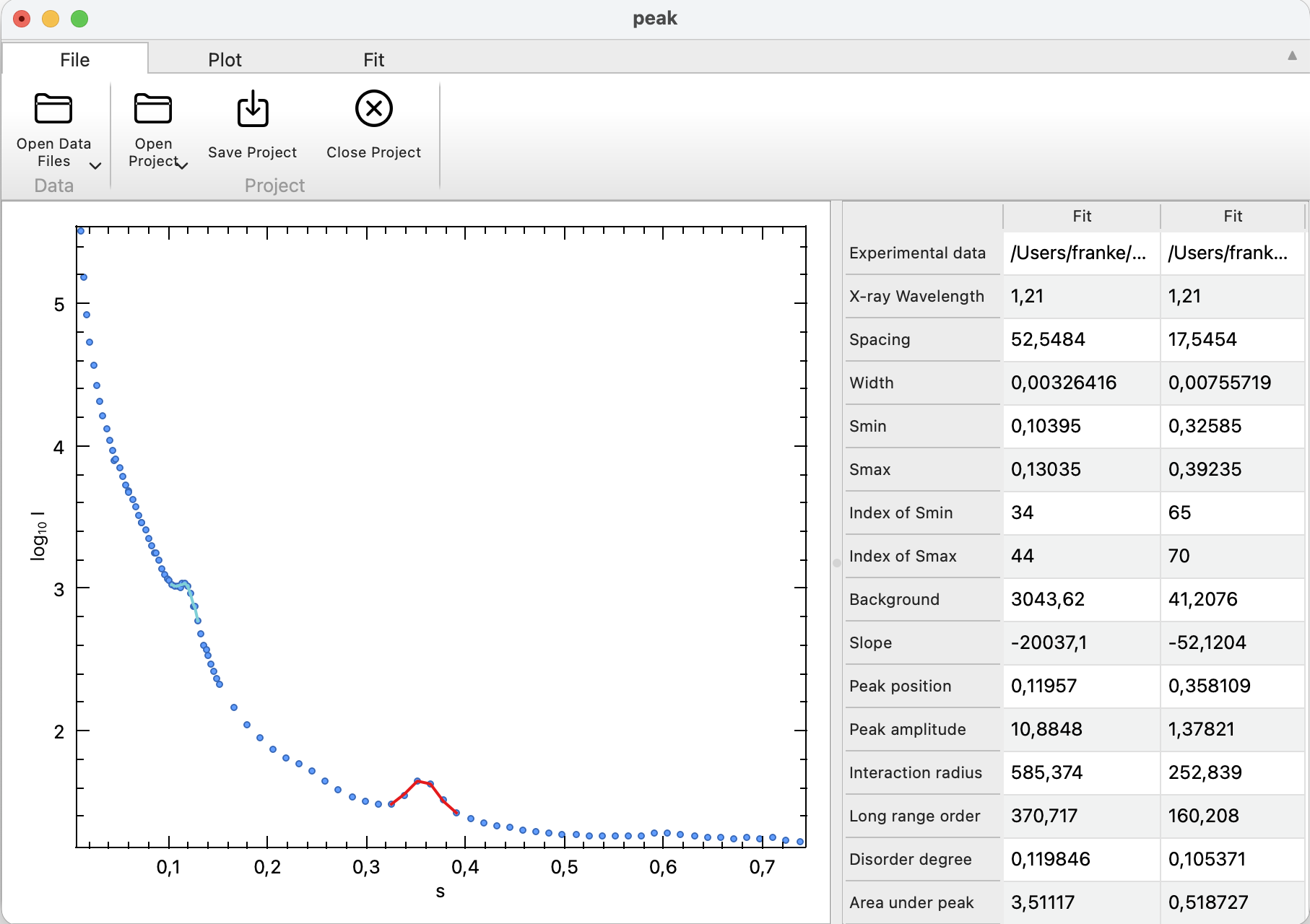
It displays the data present in the experimental SAS data (.dat) file, and allows the user to select ranges for analysis.
Only one file may be worked with at a time; the state of PEAK and all its selections may be saved as project.
All plot features are supported.
Running peak
Working with Data
PEAK displays exactly one experimental data file.
- To load a data file individually: File -> Open Data File. This adds the selected data to the current project.
Working with Projects
Projects contain information about loaded data and all plot configurations done previously. There can be only one project open at a time, and each project may contain exactly one data file.
PEAK starts with an empty project and adds the loaded data file to it.
- To load a previously saved project: File -> Open Project. Loading a new project replaces the current project.
- To save the current application state: File -> Save Project. If no project is currently active, it is saved to a new project file.
- To save the project in a new file: File -> Save Project As.
- To close the current Project: File -> Close Project. Closing a project removes all data from all plots.
- To package a project to a self-contained .zip archive: File -> Package Project
Configuration
The configuration dialog controls global options. The following settings are available:
| Name | Description |
|---|---|
| Wavelength [\(\AA\)] | X-ray wavelength \(\lambda\) used for derived parameters. |
| Fit Function | One of Gaussian, Lorentzian or Gauss-Lorentz Mixture (Pseudo-Voigt). |
Peak parameters for already selected ranges are not recalculated automatically after a configuration change. To compare fit functions, change the setting and add the same range again.
- To open the settings dialog: Peak -> Configure (Linux, Windows). On macOS, use the standard Preferences shortcut ⌘+, (peak -> Preferences).
Analysing Peaks
PEAK fits the selected \(s\)-range with a user-defined function:
- Gaussian distribution
- Lorentzian distribution
- Pseudo-Voigt, a mixture of Gaussian and Lorentzian; the Pseudo-Voigt is parameterized by \(\eta\). If \(\eta=0\), the pure Gaussian is selected; if \(\eta=1\) the pure Lorentzian is selected, and the mixture case arises for \(0.0 < \eta < 1.0\).
In all cases, a linear background component \((B + Ms)\) is assumed and a factor \(A\) is applied to scale the distribution to the data.
Therefore, the fitted model is
\[I_{\mathrm{fit}}(s) = B + M s + A \left[\eta\,L(s;\mu,\gamma) + (1-\eta)\,G(s;\mu,\sigma)\right]\]Derived quantities (using the configurable wavelength \(\lambda\)) are computed from the fitted FWHM and position:
\[\beta = 2\arcsin\!\left(\min\!\left(1,\frac{(\mu+\mathrm{FWHM}/2)\lambda}{4\pi}\right)\right) - 2\arcsin\!\left(\min\!\left(1,\frac{(\mu-\mathrm{FWHM}/2)\lambda}{4\pi}\right)\right)\] \[\cos\theta = \cos\!\left(\arcsin\!\left(\frac{\mu\lambda}{4\pi}\right)\right)\]The following values are reported for each peak:
| Parameter | Description |
|---|---|
| Experimental data | Full path to the data file. |
| X-ray wavelength | Assumed wavelength \(\lambda\), user configurable. |
| Spacing | parameter \(d\), \(d = 2\pi/\mu\), the real-space repeat distance corresponding to the peak position. |
| Width | \(\beta\) (in radians), the angular peak broadening derived from the fitted FWHM. |
| Smin | First \(s\)-value in the selected range. |
| Smax | Last \(s\)-value in the selected range. |
| Index of Smin | Integer index of the first data point in the selected range. |
| Index of Smax | Integer index of the last data point in the selected range. |
| Background | Constant offset \(B\) across the selected peak. |
| Slope | Slope \(M\) across the selected peak. |
| Peak position | Parameter \(\mu\), peak center within the selected \(s\) range. |
| Peak amplitude | Parameter \(A\), the scale factor of the normalized peak profile. |
| Interaction radius | \(R = (2\pi/5)^2\,\lambda/\beta\). |
| Long range order | \(L = \lambda / (\beta \cos\theta)\), a correlation length (order dimension) inferred from the peak width. |
| Disorder degree | \(\Delta/d = \sqrt{\beta d/\lambda}/\pi\). |
| Area under peak | integral of \(I_{\mathrm{exp}}(s)\) over the selected range minus the background. |
| Fit quality [chi^2] | reduced \(\chi^2\) statistic of the experimental data and calculated distribution. |
| Fit function | Name of the function used, user configurable. |
| Gaussian [%] | \(100(1-\eta)\). |
| Lorentzian [%] | \(100\eta\). |
- To add a new peak fit, use the Select Range mode of the plot window
- To remove a peak fit: Fit -> Remove Selection
- To edit a peak fit, remove the current selection and add a new peak with the modified range. It is not possible to add or remove individual points to a selection
- To export the analysis table: Fit -> Export. The output is a CSV formatted file; the first column is the descriptions, each following column the values of each selection
- Selecting a table column highlights the corresponding peak fit in the plot