gnom
Manual
The following sections briefly describe the method implemented in GNOM, how to run GNOM from the command-line, and the required input and generated output files.
The command-line version of GNOM described in this manual is intended primarily for scripted or batch workflows. For interactive use with immediate visual feedback, it is strongly recommended to employ the graphical wizard available in PRIMUS (Analysis -> Distance Distribution), which invokes GNOM internally.
Introduction
GNOM is an indirect transform program for small-angle scattering (SAS) data processing. It reads one-dimensional scattering curves (optionally smeared by instrumental effects) and evaluates the real-space distance distribution function \(p(r)\) for monodisperse particles, or size distribution functions for selected polydisperse systems. The recovered distribution is obtained by solving a regularized least-squares problem that balances a fit to the experimental data with smoothness and physical constraints:
The real-space distribution is related to the scattering intensity through a Fourier transform,
\[p(r) = \frac{r^2}{2 \pi^2} \int_0^\infty s^2 I(s) \frac{\sin(sr)}{sr} ds + \alpha \, S[p(r)]\]Here, \(\alpha \, S[p(r)]\) is the regularization term that penalizes non-smooth solutions. To solve this, GNOM applies Tikhonov regularization and estimates the regularization parameter \(\alpha\) automatically using perceptual criteria. Here, perceptual criteria encode a preference for smooth, non-oscillatory distributions, reflecting the empirical observation that strong high-frequency “wriggles” are usually artifacts rather than physical features. The implementation is heuristic and historically motivated; it is not a universal statistical optimum, but it has proven robust.
Further, GNOM may account for 1D slit or 2D detector smearing and merge multiple datasets collected under different experimental conditions.
System
The system type selects the assumed particle model GNOM uses when
converting SAS data into a real-space distribution. It determines
which distribution is reconstructed and which constraints are applied during regularization.
The system type is identified by numerical id, with the following ones available:
| ID | Description | Output |
|---|---|---|
| 0 | arbitrary monodisperse particles | pair distance distribution function, \(p(r)\) |
| 1 | polydisperse solid sphere | volume distribution |
| 2 | polydisperse particles with a user-supplied form factor | size distribution |
| 3 | monodisperse flattened particles | thickness distribution |
| 4 | monodisperse rod-like particles | cross-section distribution |
| 5 | polydisperse long cylinders | length distribution |
| 6 | polydisperse spherical shells | surface distribution with a relative shell thickness parameter |
system=0 is most commonly used for biological Small Angle Scattering.
Setup
The experimental setup describes how instrumental smearing is modeled during the transform (collimation geometry, beam profile, wavelength spread).
Most synchrotron beamlines will have point collimation, many lab sources may use slit collimation, neutron sources may require a spot function.
If you are unsure which setup matches your data, consult the instrument scientist or beamline staff.
Point Collimation
Point collimation assumes the measured curve is already free of instrumental smearing. If point-collimation is selected, GNOM reconstructs the real-space distribution directly from the observed data.
Slit Collimation
Slit collimation models 1D detector geometry using rectangular slits. GNOM
describes slit height and width with trapezoidal profiles defined by parameters
A (flat section width) and L (edge length), or with experimental profile
files. Wavelength spread can be included as a separate smearing component.
This setup is generally appropriate for linear detector or scanning slit systems. All slit parameters use the same units as the scattering vector in the input data.
Spot Function
Spot function is intended for 2D detectors where the scattering curve is obtained by radial averaging. GNOM reads a beam profile file containing a square matrix of primary beam intensities on the detector, radially averages and normalizes it, then uses the resulting spot function to apply smearing.
Running GNOM
Command-Line Arguments and Options
Usage:
$ gnom [OPTIONS] [SASDATA]
If GNOM is started without any arguments, it switches to the interactive dialog mode. In command-line mode, at most one file name may be provided.
GNOM accepts the following command line arguments:
| Argument | Description |
|---|---|
| SASDATA | Optional experimental SAS data (.dat) input file. |
Absolute as well as relative paths to data files are accepted. Instead of a file name, the argument may be given as ‘-‘ to read data from stdin.
GNOM recognizes the following command-line options:
| Short option | Long option | Description |
|---|---|---|
| --seed <INT> | Set the seed for the random number generator. | |
| --first <N> | First point of the data file to use (default: 1). | |
| --last <N> | Last point of the data file to use (default: all). | |
| --system <N> | System type, one of 0…6 (default: 0). System 2 (user-supplied form factor) is not supported on the command line; use interactive mode. | |
| --rmin <VALUE> | Minimum characteristic size of the selected system (default: 0.0). | |
| --rmax <VALUE> | Maximum characteristic size of the selected system (required). | |
| --rad56 <VALUE> | System-specific parameter for system 5 or 6: cylinder radius (system 5) or relative shell thickness in [0, 1] (system 6); default: 0.0. | |
| --force-zero-rmin <Y|N> | Apply the zero condition at r=rmin (default: YES). | |
| --force-zero-rmax <Y|N> | Apply the zero condition at r=rmax (default: YES). | |
| --nr <N> | Number of points in real space (default: automatic). | |
| --alpha <VALUE> | Regularization parameter alpha (default: automatic). | |
| -o | --output <FILE> | Output file name; if not specified, GNOM writes to stdout. |
| -v | --version | Print version information and exit. |
| -h | --help | Print a summary of arguments, options, and exit. |
Notes:
- only point collimation is available from the command-line. For slit or spot smearing, use the interactive configuration.
- only one experimental SAS data (.dat) file may be provided at the command-line. If data is available from different setups (e.g. SAXS+WAXS, different detector distances, point and slit collimation, etc) use interactive configuration to automatically merge.
- System 2, user-supplied form factor, is not supported on the command line; use interactive configuration instead
Interactive Configuration
GNOM enters the interactive dialog when started without command-line arguments. The questions asked depend on the configuration mode, the selected system, and the experimental setup.
The overall structure of the dialog tree:
General configuration
The following prompts are shown for all modes unless stated otherwise.
| Screen Text | Default | Description |
|---|---|---|
| Configuration Mode? | user | Select user or expert mode. Expert mode enables multiple input files, prompts for expert-criteria weights/sigmas, and other options not commonly used. |
| Screen Text | Mode | Default | Description |
|---|---|---|---|
| Number of input files | E | 1 | Number of datasets to process into a single output (defaults to 1 in user mode). Note: expert repeats the file name/first/last/setup questions for all input files. When multiple input files are supplied, GNOM scales all additional datasets to the first and merges them automatically. |
| Input data file name? | U|E | None | Absolute or relative path to a experimental SAS data (.dat) file. Asked once per input file. |
| First point to use in the data file? | U|E | 1 | Index of the first data point to be used from the most recent input file. |
| Last point to use in the data file? | U|E | last | Index of the last data point used from the most recent input file. |
| Experimental setup? | U|E | point collimation | Select point collimation, slit collimation, or spot function for the most recent input file. This selection may lead to additional questions later. See setup-specific parameters. |
| Zero condition at r=rmin | U|E | yes | Enforce \(p(r_{\min})=0\). |
| Zero condition at r=rmax | U|E | yes | Enforce \(p(r_{\max})=0\). |
| Number of points in real space? | U|E | automatic | GNOM suggests a value based on the data; maximum: 256. |
| Initial alpha (0.0 automatic)? | U|E | 0.0 | Regularization parameter \(\alpha\); use 0.0 for automatic optimization. |
| Initial random seed? | E | current time | Leave blank to use the current time. |
| Output file name? | U|E | basename.out | For a single input file, the default is the input base name with .out. For multiple input files, provide a file name. |
| Weight/sigma of DISCRP | E | 1.0 / 0.30 | Discrepancy between experimental and fitted data. |
| Weight/sigma of OSCILL | E | 3.0 / 0.60 | Oscillation/smoothness of the recovered distribution. |
| Weight/sigma of STABIL | E | 3.0 / 0.12 | Stability of the solution with respect to alpha. |
| Weight/sigma of SYSDEV | E | 3.0 / 0.12 | Systematic deviations between fit and data. |
| Weight/sigma of POSITV | E | 1.0 / 0.12 | Positivity of \(p(r)\). |
| Weight/sigma of VALCEN | E | 1.0 / 0.12 | Concentration of \(p(r)\) in the central region. |
| Weight/sigma of SMOOTH | E | 1.0 / 0.60 | Smoothness of the tail of \(p(r)\). |
System-specific parameters
After selecting the system type, GNOM asks for parameters specific to that system. All sizes use the same real-space units as the input data.
System 0: arbitrary monodisperse
| Prompt | Default | Description |
|---|---|---|
| Maximum particle diameter for p(r)? | None | Sets \(r_{\max}\) for the distance distribution. |
System 1: polydisperse spheres
| Prompt | Default | Description |
|---|---|---|
| Minimum sphere radius for p(r)? | 0.0 | Lower bound of the radius range. |
| Maximum sphere radius for p(r)? | None | Upper bound of the radius range. |
System 2: arbitrary polydisperse (user-supplied form factor)
| Prompt | Default | Description |
|---|---|---|
| Minimum characteristic size for p(r)? | None | Lower bound of the size range. |
| Maximum characteristic size for p(r)? | None | Upper bound of the size range. |
| Form Factor file name? | None | Path to a form factor file (see gnom input files). |
System 3: monodisperse flattened particles
| Prompt | Default | Description |
|---|---|---|
| Maximum particle thickness for p(r)? | None | Sets \(r_{\max}\) for thickness distribution. |
System 4: monodisperse rod-like particles
| Prompt | Default | Description |
|---|---|---|
| Maximum diameter of particle cross-section? | None | Sets \(r_{\max}\) for cross-section distribution. |
System 5: polydisperse long cylinders
| Prompt | Default | Description |
|---|---|---|
| Minimum height of cylinder? | 0.0 | Lower bound of cylinder length. |
| Maximum height of cylinder? | None | Upper bound of cylinder length. |
| Cylinder radius? | None | Fixed cylinder radius used for the distribution. |
System 6: polydisperse spherical shells
| Prompt | Default | Description |
|---|---|---|
| Minimum outer shell radius? | 0.0 | Lower bound of the outer shell radius. |
| Maximum outer shell radius? | None | Upper bound of the outer shell radius. |
| Relative shell thickness [0.0, 1.0]? | None | Relative shell thickness (0.0 means infinitely thin). |
Setup-specific parameters
Experimental setup prompts are shown once per input file. Note that is expressly expected that multiple inputs for the same system have different instrumental setup.
Point collimation
No additional parameters are requested.
Slit collimation
Slit smearing uses trapezoidal slit profiles described by parameters A
(flat section width) and L (edge length). Profiles can also be supplied from
experimental files.
| Prompt | Default | Description |
|---|---|---|
| Slit height setup? | parametrized slit profile | Choose none, parametrized slit profile, or experimental slit profile. |
If parametrized slit profile is selected:
| Prompt | Default | Description |
|---|---|---|
| Slit height parameter A? | 0.0 | Flat section width AH for the slit-height profile (see Fig. 1). |
| Slit height parameter L? | 0.0 | Edge length LH for the slit-height profile (see Fig. 2, must be <= AH). |
| Slit width parameter A? | 0.0 | Flat section width AW for the slit-width profile (see Fig. 3). |
| Slit width parameter L? | 0.0 | Edge length LW for the slit-width profile (see Fig. 4, must be <= AW). |
The case of “infinitely long slit” can be covered, e.g., by putting AH=\(s_{\max}\), LH=0.0, where \(s_{\max}\) is the momentum transfer of the last data point.
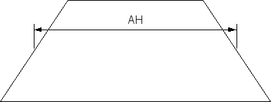
Figure 1 Projection of the beam height in the detector plane.
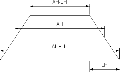
Figure 2 Half of the height difference between top and bottom edge of beam projection on the detector.
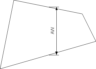
Figure 3 Projection of the beam width in the detector plane.
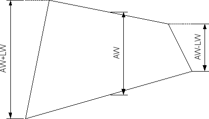
Figure 4 Half of the width difference between top and bottom edge of beam projection on the detector.
If experimental slit profile is selected:
| Prompt | Default | Description |
|---|---|---|
| Slit height experimental profile file? | None | File with an experimentally measured slit-height profile (see input files). |
| Slit width experimental profile file? | None | File with an experimentally measured slit-width profile. |
Either is followed by:
| Prompt | Default | Description |
|---|---|---|
| Wavelength distribution setup? | parametrized wavelength profile | Choose none, parametrized wavelength profile, or experimental wavelength profile. |
If parametrized wavelength profile is selected:
| Prompt | Default | Description |
|---|---|---|
| FWHM of wavelength distribution [0.0-1.0)? | 0.0 | Relative Full Width at Half-Maxium used for a parametrized wavelength profile. FWHM=0 means monochromatic radiation. |
If experimental wavelength profile is selected:
| Prompt | Default | Description |
|---|---|---|
| Wavelength distribution experimental profile file? | None | File with an experimentally measured wavelength profile. |
Spot function
Spot function uses a 2D beam profile measured on the detector and applies smearing based on its circularly averaged spot function.
| Prompt | Default | Description |
|---|---|---|
| Beam profile file name? | None | File containing the beam profile matrix (see input files). |
If the beam profile file includes a wavelength profile, GNOM uses it directly. Otherwise, it prompts for the wavelength distribution using the same options as in slit collimation.
Runtime Output
GNOM does not produce a separate runtime log. Instead, all information about a run is written to the regularised SAS data (.out), or to standard output if no output file name is specified (command-line only).
The regularised SAS data (.out) file contains
the runtime configuration used for the calculation, followed by the
results of the parameter search. The angular and real-space ranges are
quoted, together with a Total Estimate, a qualitative assessment
based on internal perceptual criteria that serves as a quick sanity
check rather than a strict statistical test.
Finally, the experimental input data are listed together with the orresponding smeared and desmeared theoretical curves calculated from the specified instrument setup and the final distribution function.
gnom Input Files
Experimental Data
GNOM expects background-subtracted experimental SAS data (.dat) files as input.
At least one file is required, but GNOM can make use of multiple data of the same system, recorded with different setups. The data will be automatically scaled and merged. This is preferable over manual merging before running GNOM.
User-defined Form-factor
If setup=2 is selected, a form-factor file with the same
format as experimental SAS data (.dat),
but without experimental errors, has to be provided.
Experimental Slit Profile
Experimental slit profiles are provided in the same format as experimental SAS data (.dat). They are expected in the same units as experimental data.
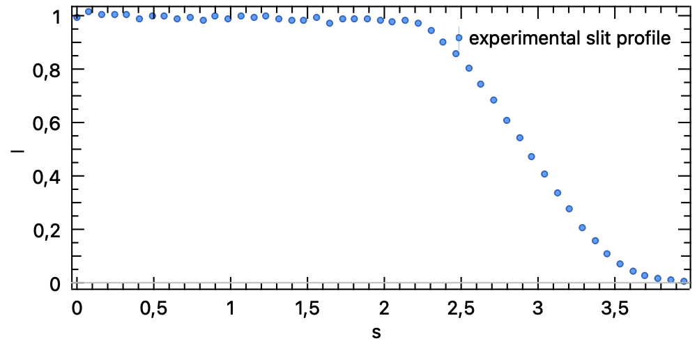
Figure 5 Example of an experimental slit profile, internally mirrored to negative values.
Beam profile (spot function)
For the spot function setup, GNOM expects a beam profile file describing the primary beam intensity on the detector plane. The file stores a square matrix and may optionally include a wavelength profile. The first line contains the matrix size and an optional scaling factor:
NB [TRANS]
NB is the number of rows and columns. TRANS relates the detector step size
to the angular step in the experimental curve (TRANS = DetSt / DeltaS). If
omitted, TRANS=1 is assumed.
The next NB lines must contain NB numbers each (the beam profile matrix).
Example of a valid spot function:
7, 0.8
             0.,  1.,   2.,   4.,   2.,  1.,  0.,
             1.,  5.,  72., 238.,  72.,  5.,  1.,
             2., 72., 765.,1836., 765., 72.,  2.,
             4.,238.,1836.,3781.,1836.,238.,  4.,
             2., 72., 765.,1836., 765., 72.,  2.,
             1.,  5.,  72., 238.,  72.,  5.,  1.,
             0.,  1.,   2.,   4.,   2.,  1.,  0.
After this, an optional wavelength profile can be appended in the format:
NW WL1 DLAM
w1 w2 ... wNW
where NW is the number of wavelength points, WL1 is the starting
wavelength, DLAM the increment, and the following line lists the weights. If
this section is missing, GNOM prompts for a wavelength distribution.
gnom Output Files
GNOM writes regularised SAS data (.out).
Examples
These examples highlight the differences between instrumental setups.
Point Collimation: Arbitrary Monodisperse Particles
Distance distribution \(p(r)\) from monodisperse lysozyme data with known \(D_{\max}\):
$ gnom lyzexp.dat --rmax=50 --output=lyzexp.out
Slit Collimation: Polydisperse spheres
The command-line does not allow arbitrary instrumental setups, hence
use interactive configuration. Here there are two input files,each
with its respective setup: one with infinitly long slits, another
with wavelength smearing. Result is written to run12.out.
$ gnom
Configuration Mode? Select one of: (e) expert, (u) user (default:
user) ................................................................ : e
Number of input files (default: 1) ................................... : 2
Input data file name? ................................................ : run1.dat
First point to use in the data file? (default: 1) .................... : 1
Last point to use in the data file? (default: 50) .................... : 50
Experimental setup? Select one of: (0) point collimation, (1) slit
collimation, (2) spot function (default: point collimation) .......... : 1
Slit height setup? Select one of: (0) none, (1) parametrized slit
profile, (2) experimental slit profile (default: parametrized slit
profile) ............................................................. : 1
Slit height parameter A? (default: 0.00) ............................. : 0.4
Slit height parameter L? (default: 0.00) ............................. : 0.2
Slit width setup? Select one of: (0) none, (1) parametrized slit
profile, (2) experimental slit profile (default: parametrized slit
profile) ............................................................. : 0
Wavelength distribution setup? Select one of: (0) none, (1)
parametrized wavelength profile, (2) experimental wavelength profile
(default: parametrized wavelength profile) ........................... : 0
Input data file name? ................................................ : run2.dat
First point to use in the data file? (default: 1) .................... : 1
Last point to use in the data file? (default: 71) .................... : 71
Experimental setup? Select one of: (0) point collimation, (1) slit
collimation, (2) spot function (default: point collimation) .......... : 1
Slit height setup? Select one of: (0) none, (1) parametrized slit
profile, (2) experimental slit profile (default: parametrized slit
profile) ............................................................. : 0
Slit width setup? Select one of: (0) none, (1) parametrized slit
profile, (2) experimental slit profile (default: parametrized slit
profile) ............................................................. : 0
Wavelength distribution setup? Select one of: (0) none, (1)
parametrized wavelength profile, (2) experimental wavelength profile
(default: parametrized wavelength profile) ........................... : 1
FWHM of wavelength distribution [0.0-1.0)? (default: 0.00) ........... : 0.1
System type? Select one of: (0) arbitrary monodisperse, (1)
polydisperse spheres, (2) arbitrary polydisperse, (3) monodisperse
flat, (4) monodisperse rods, (5) polydisperse long cylinders, (6)
polydisperse spherical shells (default: arbitrary monodisperse) ...... : 1
Minimum sphere radius for p(r)? (default: 0.00) ...................... : 50
Maximum sphere radius for p(r)? ...................................... : 150
Zero condition at r=rmin (default: yes) .............................. :
Zero condition at r=rmax (default: yes) .............................. :
 Weight/sigma of DISCRP .... <        1.000,      0.3000 >:
 Weight/sigma of OSCILL .... <        3.000,      0.6000 >:
 Weight/sigma of STABIL .... <        3.000,      0.1200 >:
 Weight/sigma of SYSDEV .... <        3.000,      0.1200 >:
 Weight/sigma of POSITV .... <        1.000,      0.1200 >:
 Weight/sigma of VALCEN .... <        1.000,      0.1200 >:
 Weight/sigma of SMOOTH .... <        1.000,      0.6000 >:
Number of points in real space? (default: 88) ........................ :
Initial alpha (0.0 automatic)? (default: 0.00) ....................... :
Initial random seed? (default: use current time) ..................... :
Output file name? .................................................... : run12.out
Spot Function: Arbitrary Monodisperse Particles
The command-line does not allow arbitrary instrumental setups, hence use interactive configuration. Here there are two input files,each with its respective setup: both collected at a neutron source, one at a distance of 10m, the other at a distance of 3m.
$ gnom
Configuration Mode? Select one of: (e) expert, (u) user (default:
user) ................................................................ : e
Number of input files (default: 1) ................................... : 2
Input data file name? ................................................ : h10100.dat
First point to use in the data file? (default: 1) .................... :
Last point to use in the data file? (default: 33) .................... :
Experimental setup? Select one of: (0) point collimation, (1) slit
collimation, (2) spot function (default: point collimation) .......... : 2
Beam profile file name? .............................................. : spot10.dat
Wavelength distribution setup? Select one of: (0) none, (1)
parametrized wavelength profile, (2) experimental wavelength profile
(default: parametrized wavelength profile) ........................... : 1
FWHM of wavelength distribution [0.0-1.0)? (default: 0.00) ........... : 0.08
Input data file name? ................................................ : h03100.dat
First point to use in the data file? (default: 1) .................... :
Last point to use in the data file? (default: 32) .................... :
Experimental setup? Select one of: (0) point collimation, (1) slit
collimation, (2) spot function (default: point collimation) .......... : 2
Beam profile file name? .............................................. : spot3.dat
Wavelength distribution setup? Select one of: (0) none, (1)
parametrized wavelength profile, (2) experimental wavelength profile
(default: parametrized wavelength profile) ........................... : 1
FWHM of wavelength distribution [0.0-1.0)? (default: 0.00) ........... : 0.08
System type? Select one of: (0) arbitrary monodisperse, (1)
polydisperse spheres, (2) arbitrary polydisperse, (3) monodisperse
flat, (4) monodisperse rods, (5) polydisperse long cylinders, (6)
polydisperse spherical shells (default: arbitrary monodisperse) ...... : 0
Maximum particle diameter for p(r)? .................................. : 800
Zero condition at r=rmin (default: yes) .............................. :
Zero condition at r=rmax (default: yes) .............................. :
 Weight/sigma of DISCRP .... <        1.000,      0.3000 >:
 Weight/sigma of OSCILL .... <        3.000,      0.6000 >:
 Weight/sigma of STABIL .... <        3.000,      0.1200 >:
 Weight/sigma of SYSDEV .... <        3.000,      0.1200 >:
 Weight/sigma of POSITV .... <        1.000,      0.1200 >:
 Weight/sigma of VALCEN .... <        1.000,      0.1200 >:
 Weight/sigma of SMOOTH .... <        1.000,      0.6000 >:
Number of points in real space? (default: 64) ........................ :
Initial alpha (0.0 automatic)? (default: 0.00) ....................... :
Initial random seed? (default: use current time) ..................... :
Output file name? .................................................... : h1003.out